Drosophila LIF Brain Computational Model: From Connectome to Functional Prediction

A summary of the paper:
Shiu, P.K., Sterne, G.R., Spiller, N. et al. A Drosophila computational brain model reveals sensorimotor processing. Nature 634, 210–219 (2024). https://doi.org/10.1038/s41586-024-07763-9

2025-07-30

Introduction

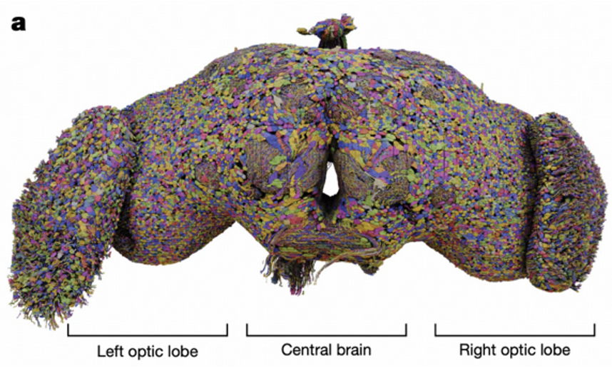
The year 2024 marks a milestone in neuroscience with the publication of the complete neuronal wiring diagram of an adult female Drosophila melanogaster brain by Dorkenwald and colleagues. This groundbreaking research encompasses 139,255 neurons and 5.45×10⁷ chemical synapses, representing the first connectome resource covering the entire brain. This achievement not only provides a valuable data foundation for neuroscience research but also opens new pathways for understanding how the brain works.

When we discuss neuron models, we're essentially talking about how to transform complex biological phenomena into computable mathematical expressions. Biological neuron models, also known as spiking neuron models, focus on describing how cell membrane potential changes over time. These changes aren't random but follow strict physical laws, much like current flow in electrical circuits.

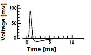
Neuron models can be broadly categorized into two types: electrical input-output membrane voltage models that process external current stimulation $I_{\text{in}}(t)$ or voltage stimulation $V_{\text{in}}(t)$ and output membrane voltage $V(t)$ or action potential trigger timing $t_{\text{spike}}$, and natural stimulus or pharmacological input neuron models that handle external natural stimuli such as light, sound $S(t)$ or chemical concentration $C(t)$ and output action potential probability $P_{\text{spike}}(t)$. Both model types have their applications but aim to capture the essential characteristics of neuronal behavior.

LIF Model: Leaky Integrate-and-Fire Model

Basic Principles

Among various neuron models, the LIF (Leaky Integrate-and-Fire) model has gained popularity due to its simplicity and practicality. This model cleverly simplifies neurons into resistor-capacitor (RC) circuits, where membrane resistance and capacitance correspond to the passive electrical properties of neurons.

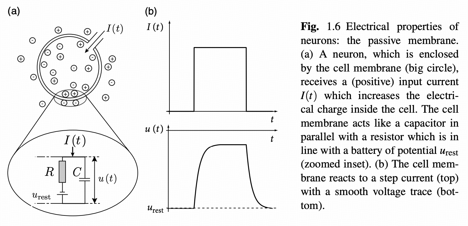
From a physics perspective, the neuronal membrane can be viewed as a capacitor capable of storing charge and generating potential differences. Simultaneously, various ion channels exist on the membrane, acting as resistors that control ion flow. When external stimuli act on neurons, these electrical components work together to produce complex potential changes.

Treating neurons as resistor-capacitor (RC) circuits, where resistance $R_{\text{mbr}}$ represents membrane resistance and capacitance $C_{\text{mbr}}$ represents membrane capacitance. The current equation is:

$$I(t)=I_R+I_C=\frac{v_R}{R_{\text{mbr}}}+C_{\text{mbr}}\frac{dv}{dt}$$

Mathematical Derivation

The mathematical expression of the LIF model is relatively concise but contains profound physical meaning. By introducing the membrane time constant $T_{\text{mbr}}=R_{\text{mbr}}{C}_{\text{mbr}}$, we can simplify complex differential equations into more manageable forms. This time constant reflects how quickly the neuronal membrane responds to potential changes and is a key parameter for understanding neuronal dynamic behavior.

Introducing leaky integrator $T_{\text{mbr}}=R_{\text{mbr}}{C}_{\text{mbr}}$, defined as membrane time constant:

$$T_{\text{mbr}}\frac{dv}{dt}=-v(t)+R_{\text{mbr}}I(t)$$

When we consider the resting potential $V_{\text{resting}}$, let $v_R=v(t)-V_{\text{resting}}$:

$$T_{\text{mbr}}\frac{dv}{dt}=-(v(t)-V_{\text{resting}})+R_{\text{mbr}}I(t)$$

The conditions for spike generation are also important components of the model. When membrane potential reaches the threshold, neurons generate action potentials, which is the basic way neurons transmit information. After a spike, membrane potential resets to a specific value, and neurons enter a refractory period during which they cannot generate new spikes.

$V_{\text{threshold}}$ is the spike threshold, $V_{\text{reset}}$ is the post-spike reset potential, and at spike generation time $t^{(f)}$:

$$v(t^{(f)})=V_{\text{threshold}},\underset{\delta \to 0;\delta >0}{lim}v(t^{(f)}+\delta )=V_{\text{reset}}$$

Network Model

While individual neuron behavior is important, the true charm of the brain lies in the complex connections between neurons. In network models, each neuron receives inputs from multiple presynaptic neurons, which are weighted and summed through synaptic weights to ultimately determine the neuron's output.

The total input current to neuron $i$ is the sum of all current pulses:

$$I_i(t)=\sum _j{w}_{ij}\sum _f\alpha (t-t_j^{(f)})$$

Where $w_{ij}$ is the synaptic efficacy from $j\to i$.

$\alpha$-synapse dynamics uses the following exponential decay function for modeling:

$$\alpha (s)=\frac{q}{\tau }{e}^{-s/\tau }\mathrm{\Theta }(s);\mathrm{\Theta }(s)=\{\begin{array}{ll}1,& s\ge 0\\ 0,& s<0\end{array}$$

$\mathrm{\Theta }(s)$ is the Heaviside step function, $\tau$ is the synaptic decay time scale, and $q$ represents the strength of the synaptic current pulse generated by presynaptic neuron $j$ firing.

Synaptic dynamics is another important concept in network models. When presynaptic neurons generate spikes, they produce current pulses in postsynaptic neurons, with pulse strength decaying over time. This decay characteristic enables neuronal networks to exhibit rich dynamic behaviors, from simple synchronous oscillations to complex chaotic patterns.

Personal Derivation

Through Laplace transformation, we can obtain analytical solutions for neuronal membrane potential changes. This solution reveals how neurons respond to synaptic inputs and how different time constants affect neuronal response characteristics. Although the derivation process is somewhat complex, the result is very intuitive: membrane potential changes are the superposition of multiple exponential decay functions, each corresponding to a synaptic input.

Each neuron is simplified to emit one pulse at $t=0$, let $u_i=v_i-V_{\text{resting}}$, then:

$$T_{\text{mbr}}\frac{d{u}_i}{dt}=-u_i+R_{\text{mbr}}\sum _j{w}_{ij}\frac{q}{\tau }{e}^{-t/\tau }\mathrm{\Theta }(t)$$

Taking Laplace transform on both sides, with initial value $u_i(0)=0$:

$$\begin{array}{rl}{T}_{\text{mbr}}s{U}_i(s)& =-U_i(s)+R_{\text{mbr}}\sum _j\frac{w_{ij}q}{\tau }\frac{1}{s+\frac{1}{\tau }}\\ U_i(s)& =\frac{R_{\text{mbr}}}{T_{\text{mbr}}s+1}\sum _j\frac{w_{ij}q}{\tau }\frac{1}{s+\frac{1}{\tau }}\end{array}$$

Defining connection weight $w_{j,i}={\displaystyle \frac{R_{\text{mbr}}{w}_{ij}{q}_{ij}}{T_{\text{mbr}}}}$, then:

$$U_i(s)=\sum _j\frac{w_{j,i}}{\tau }\frac{1}{(s+\frac{1}{T_{\text{mbr}}})(s+\frac{1}{\tau })}=\sum _j\frac{w_{j,i}}{1-\tau /T_{\text{mbr}}}(\frac{1}{s+\frac{1}{T_{\text{mbr}}}}-\frac{1}{s+\frac{1}{\tau }})$$

Through inverse Laplace transformation, we obtain the membrane potential change $u_i(t)$ of neuron $i$:

$$v_i(t)-V_{\text{resting}}=u_i(t)=\sum _j\frac{w_{j,i}}{1-\frac{\tau }{T_{\text{mbr}}}}(\exp (-\frac{t}{T_{\text{mbr}}})-\exp (-\frac{t}{\tau }))\mathrm{\Theta }(t)$$

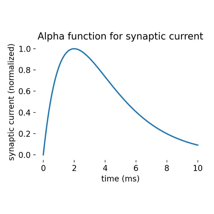
This analytical solution not only helps us understand neuronal behavior but also provides a theoretical foundation for subsequent network simulations. By adjusting different parameters, we can simulate various neuronal response patterns, thereby better understanding how neural circuits work.

Model in the Paper

Drosophila LIF Brain Model

Based on the adult Drosophila central brain connectome and neurotransmitter predictions, Shiu and colleagues created a comprehensive LIF model. This model not only reproduces known neural circuit functions but, more importantly, predicts new neural mechanisms, providing guidance for experimental research.

The model demonstrates excellent predictive capabilities in two classic systems: the feeding initiation circuit and the antennal grooming circuit. In the feeding initiation circuit, the model accurately predicts key response neurons under different taste stimuli such as sugar, water, and bitter taste. In the antennal grooming circuit, the model successfully identifies known key neurons and reveals differential mechanisms of different mechanosensory neuron subpopulations in circuit activation.

Model Parameters

The model's success largely depends on reasonable parameter settings. The LIF model used in the paper contains two main differential equations: one describing membrane potential changes and another describing synaptic conductance decay. These two equations are coupled and jointly determine the dynamic behavior of neurons.

Considering the potential changes brought by each presynaptic neuron $j$ separately, we can construct a system of differential equations:

LIF model used in the paper:

$$\begin{array}{rl}\frac{d{v}_i}{dt}& =\frac{g_i-(v_i-V_{\text{resting}})}{T_{\text{mbr}}}\\ \tau \frac{d{g}_i}{dt}& =-g_i\\ g_i& \leftarrow g_i+w_{j,i}\text{upon spike from synapse }j\end{array}$$

Using tools like Wolfram Alpha to solve, we can verify that the form of $v_i(t)$ is the same as mentioned above.

The paper references the derivation in Brian 2 documentation, but the ODE form given in the documentation is inconsistent with the above system (not distinguishing between membrane time constant $T_{\text{mbr}}$ and synaptic decay time constant $\tau$), so I attempted to provide the derivation of the model in the paper:

$$\begin{array}{rl}\tau \frac{dv}{dt}& =V_{\mathrm{rest}}-v+g\\ \tau \frac{dg}{dt}& =-g\\ g& \leftarrow g+w_i\text{upon spike from synapse }i\end{array}$$

Parameter Name	Symbol	Value	Parameter Name	Symbol	Value
Resting Potential	$V_{\text{resting}}$	$-52\text{mV}$	Post-spike Reset Potential	$V_{\text{reset}}$	$-52\text{mV}$
Spike Threshold	$V_{\text{threshold}}$	$-45\text{mV}$	Membrane Resistance	$R_{\text{mbr}}$	$10{\text{Kohm·cm}}^2$
Refractory Period	$T_{\text{refractory}}$	$2.2\text{ms}$	Membrane Capacitance	$C_{\text{mbr}}$	$2\mu {\text{F·cm}}^{-2}$
Membrane Time Constant	$T_{\text{mbr}}$	$C_{\text{mbr}}\times R_{\text{mbr}}$	Synaptic Decay Time Scale	$\tau$	$5\text{ms}$
Spike to Membrane Potential Change Time Delay	$T_{\text{dly}}$	$1.8\text{ms}$	Synaptic Weight	$W_{\text{syn}}$	$0.275\text{mV}$
Presynaptic Neuron Set Generated Conductance	$g_i$

The only free parameter in the model is the synaptic weight $W_{\text{syn}}$, with all other parameters determined from previous research. The connection weight $w_{j,i}$ between neuron $j$ and neuron $i$ is the synaptic connection weight from the Flywire connectome multiplied by $W_{\text{syn}}$ (if $j$ is excitatory) or $-W_{\text{syn}}$ (if $j$ is inhibitory).

This design ensures the model's biological reasonableness while providing sufficient flexibility to adapt to different neural circuits.

Brian 2 Simulation

Model implementation relies on powerful computational tools. Brian 2 is a Python library specifically designed for neuroscience simulation, supporting simulation through ODE equation systems, making it ideal for LIF model implementation. Each experiment conducts 30 simulations, with each simulation lasting 1000 milliseconds, ensuring result reliability while controlling computational costs.

def run_trial(exc, exc2, slnc, path_comp, path_con, params):
    # Step 1: Create the LIF model based on connectome data
    neu, syn, spk_mon = create_model(path_comp, path_con, params)

    # Step 2: Create Poisson input for specified neurons
    poi_inp, neu = poi(neu, exc, exc2, params)

    # Step 3: Silence specified neurons
    syn = silence(slnc, syn)

    # Step 4: Run the simulation
    net = Network(neu, syn, spk_mon, poi_inp)
    net.run(duration=params["t_run"])

    # Step 5: Get spike data
    spk_trn = get_spk_trn(spk_mon)

    return spk_trn

During simulation, each neuron's state continuously updates according to differential equations, synaptic connections are determined based on connectome data, and the entire network exhibits complex dynamic behaviors. By analyzing these behaviors, we can gain deep insights into how neural circuits work.

Feeding Initiation Circuit Research

Circuit Overview

The feeding initiation circuit is a classic system in Drosophila behavior research. When Drosophila perceives sugar water, this circuit activates specific neurons to initiate feeding behavior. Several important reasons exist for selecting this circuit: first, it's completely within the field of view of Flywire electron microscopy, allowing us to obtain complete connection information; second, this circuit has been extensively studied in the literature, providing many known results for model validation.

Sugar GRN Research

Experimental Design

In Drosophila's taste system, there are four main types of gustatory receptor neurons (GRNs): sugar, water, bitter taste, and ionotropic receptor Ir94e-labeled GRNs. When Drosophila encounters sugar, sugar GRN activation leads to activation of proboscis motor neurons through a series of interneurons, causing proboscis extension.

We particularly focus on the MN9 neuron that controls proboscis elevation, as its activity directly reflects the activation state of the feeding initiation circuit. Through computer simulation, we can observe MN9 neuron response patterns under different sugar GRN activation frequencies.

Simulation Results

Simulation results show a clear positive correlation between sugar GRN activation frequency and MN9 neuron firing frequency. When sugar GRNs activate at 10Hz, MN9 neurons produce relatively low responses; when frequency increases to 200Hz, MN9 neuron responses significantly enhance.

# define inputs
# list of the labellar sugar-sensing gustatory receptor neurons on right hemisphere
neu_sugar = [
    720575940624963786, 720575940630233916, 720575940637568838, 720575940638202345, 720575940617000768,
    720575940630797113, 720575940632889389, 720575940621754367, 720575940621502051, 720575940640649691,
    720575940639332736, 720575940616885538, 720575940639198653, 720575940620900446, 720575940617937543,
    720575940632425919, 720575940633143833, 720575940612670570, 720575940628853239, 720575940629176663,
    720575940611875570,
]

# frequencies
freqs =  [ *range(10, 201, 10) ]

# run siumulations
# Calculate which neurons respond to sugar GRN firing at the specified frequencies.
for f in freqs:

    params['r_poi'] = f * Hz
    
    run_exp(exp_name='sugarR_{}Hz'.format(f), neu_exc=neu_sugar, params=params, **config)

More interestingly, simulation also revealed an important phenomenon: unilateral sugar GRN activation not only activates ipsilateral MN9 neurons but also more strongly activates contralateral MN9 neurons. This cross-activation mechanism helps Drosophila extend toward food sources, representing a meaningful biological discovery.

Network Prediction

As sugar GRN activation frequency increases, not only does MN9 neuron activity enhance, but other motor neurons like MN6, MN8, and MN11 also show corresponding increases. This indicates that sugar taste detection activates a complex network rather than a simple linear pathway.

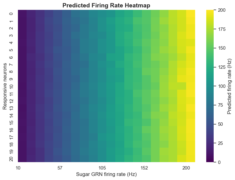
The model predicts that under 10Hz sugar GRN activation, 45 neurons will respond; under 200Hz activation, the number of responding neurons increases to 455. This order-of-magnitude change demonstrates that neural circuits have significant dynamic characteristics, able to adjust their response range based on input intensity.

Key Neuron Identification

To identify neurons most important for sugar taste response, we adopted a systematic silencing approach. After activating sugar GRNs, we individually silenced each of the 200 neurons most responsive to sweetness, observing changes in MN9 neuron activity.

# Run simulations at different frequencies
for freq in freqs:
    params['r_poi'] = freq * Hz

    for i in id_top200:
        run_exp(exp_name='sugarR-silencing{}_{}_Hz'.format(i, freq), neu_exc=neu_sugar, neu_slnc=[ i ], params=params, **config)

Analysis results show that individual neuron silencing has the greatest impact when sugar GRNs are activated at low frequencies, with circuit redundancy significantly increasing as stimulus intensity increases. This redundant design may be an important guarantee for biological system robustness.

Ultimately, we identified 47 neurons predicted to respond to sugar and sufficient to initiate feeding, with 14 being essential for MN9 neuron activity. These key neuron identifications provide important clues for understanding feeding initiation mechanisms.

Optogenetic Validation

Computational model predictions require experimental validation. We used optogenetic methods, activating specific neurons to observe Drosophila behavioral responses. This approach independently evaluates computational model accuracy, providing direct evidence for model effectiveness.

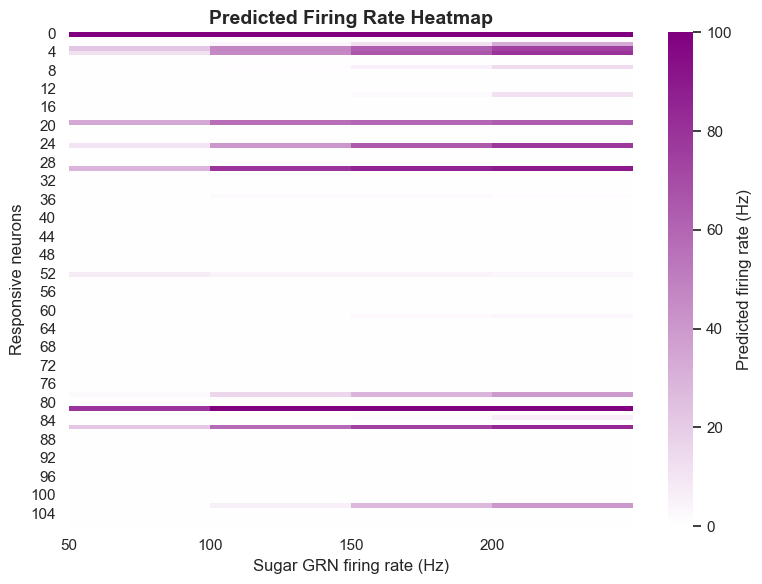
Validation results show the model excels at predicting MN9 neuron activation. Among 11 neuron types predicted to activate MN9, 10 actually trigger proboscis extension during optogenetic activation, with a true positive rate of approximately 90.91%. Among 95 neuron types predicted not to activate MN9, 91 actually don't trigger proboscis extension during optogenetic activation, with a true negative rate of approximately 95.79%.

Bitter and Ir94e GRNs

Bitter Inhibition Mechanism

Bitter taste plays an important inhibitory role in Drosophila's taste system. Using calcium imaging, we found that bitter GRN activation inhibits the sugar pathway at the pre-motor neuron level. The computational model also confirms this: when bitter taste detection is added to sugar GRN activation, it leads to inhibition of MN6 and MN9.

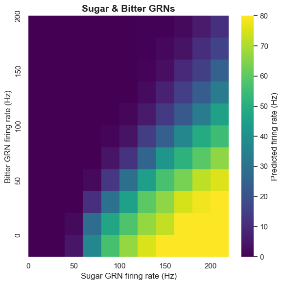
This inhibition mechanism has important biological significance. In nature, bitter taste is usually associated with toxic substances. By inhibiting feeding behavior, Drosophila can avoid ingesting harmful substances. Our model successfully captures this protective mechanism.

Ir94e GRN Function

The role of ionotropic receptor Ir94e-labeled GRNs in the proboscis has been unclear. The computational model predicts that Ir94e GRN activation inhibits MN9 neuron activity. This prediction was validated through optogenetic experiments.

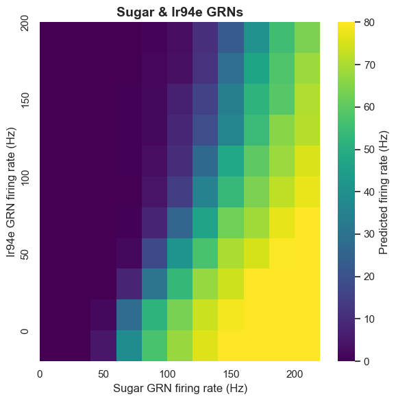
Experiments prove that Ir94e GRN activity indeed inhibits proboscis extension, but this inhibition is limited and cannot completely suppress proboscis extension to strong sugar stimulation. This discovery not only validates the model's predictive ability but also reveals a new regulatory mechanism in the taste system.

Water GRN

Water-Sugar Pathway Analysis

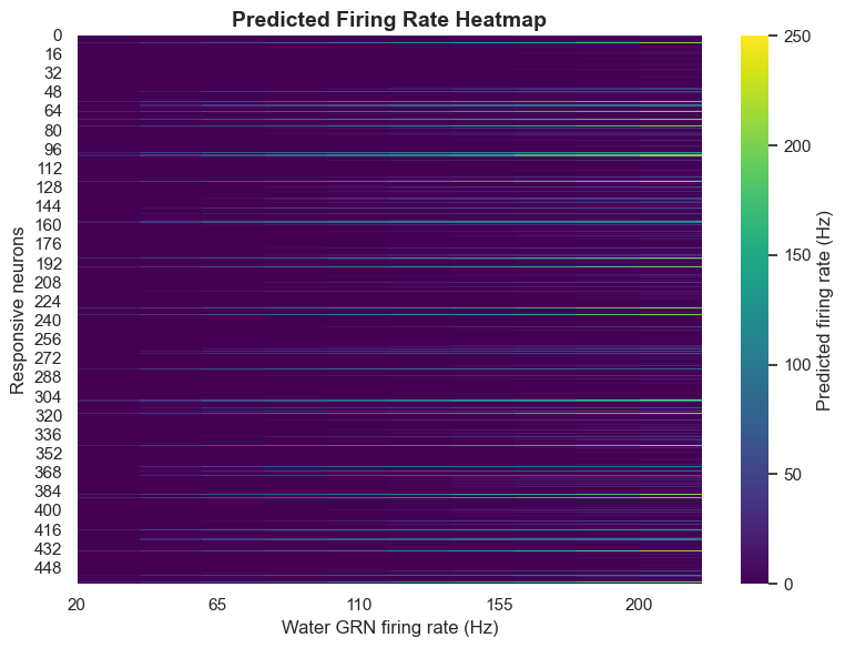
Water GRN research adopted the same analysis method as sugar GRNs. By stimulating water GRNs, we calculated responding neuron firing frequencies, identified neuron subsets capable of activating MN9, and analyzed these neurons' effects on MN9 activity.

Pathway Sharing Mechanism

The extent to which sugar and water GRNs activate different or shared pathways is an interesting question. By analyzing MN9 firing patterns under combined sugar and water activity, we discovered some important patterns.

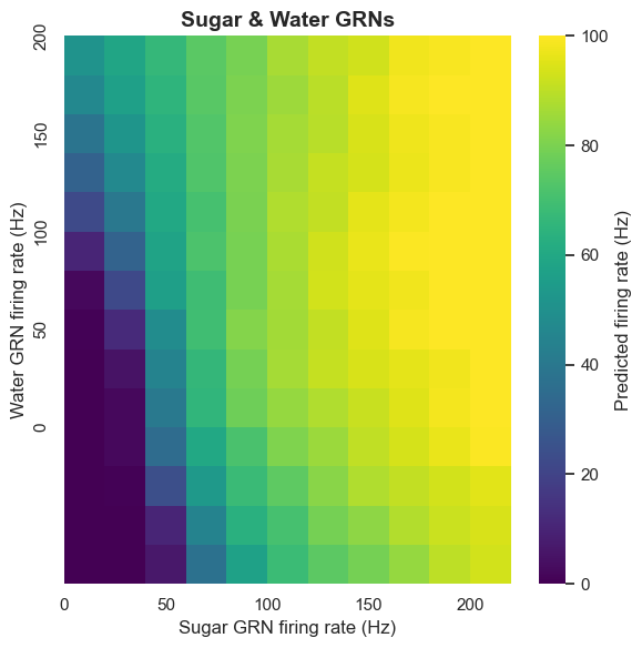
The computational model shows that water GRNs activate many downstream neurons with high overlap with neurons activated by sugar GRNs. Conversely, they have low overlap with bitter and Ir94e-related neurons. This pattern indicates that water and sugar pathways share common components at least partially, forming a rewarding ingestion pathway.

Antennal Grooming Circuit Research

Circuit Structure

Antennal grooming is another important behavior in Drosophila, involving mechanosensory neurons, interneurons, and descending neurons on the antennae. This circuit has been extensively studied in the literature, providing us with an excellent platform to validate model capabilities.

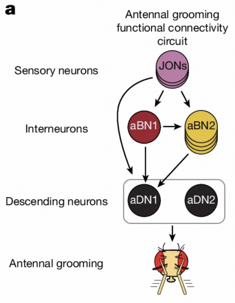
Our model successfully validates this circuit's structure, proving that computational models are sufficient to provide insights into complex circuits. This validation not only enhances our confidence in model reliability but also lays the foundation for subsequent research.

JONs and aDN1 Analysis

Using the same method as sugar GRN analysis, we analyzed JONs (Johnston's organ neurons) affecting aDN1. These neurons are located in Drosophila's antennae, responsible for detecting mechanical stimuli.

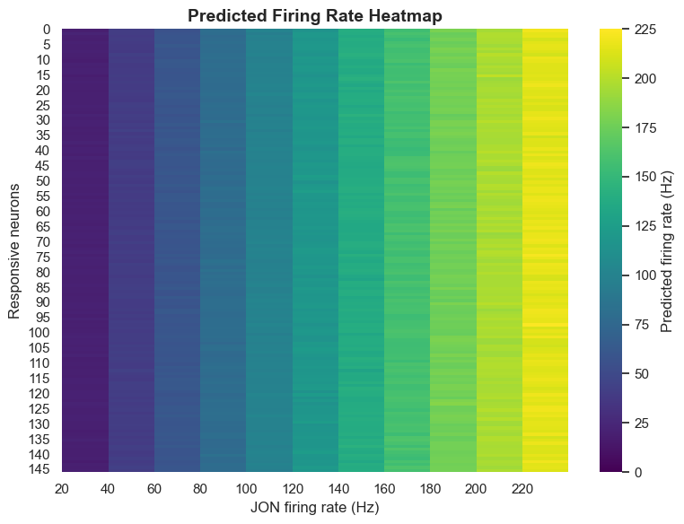
Analysis results show that the computational model can identify each key node member of the antennal grooming circuit solely from knowledge of sensory input and descending output. This capability demonstrates that connectome data indeed contains sufficient information to predict neural circuit functions.

JON Subpopulation Differences

JONs in the antennae can be divided into different subpopulations that may have functional differences. Connectome data shows that both JO-CE and JO-F neurons synapse to aBN1, but the computational model predicts they will produce different effects.

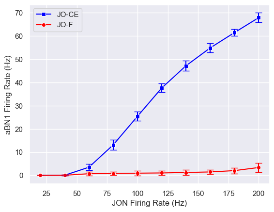
The model predicts that JO-CE neurons will trigger strong aBN1 activity, while JO-F neurons will not. This prediction was validated through optogenetic methods, further proving the model's effectiveness.

More interestingly, we identified 3 putative inhibitory neurons directly synapsing with JO-F neurons. When these inhibitory neurons are silenced, JO-F neurons can activate aBN1. This discovery not only validates the model's predictions but also reveals a new regulatory mechanism in the antennal grooming circuit.

Conclusion and Outlook

Main Contributions

Through in-depth analysis of the Flywire connectome combined with the LIF model, we successfully constructed a computational model of the Drosophila brain. This model not only reproduces known neural circuit functions but, more importantly, predicts new neural mechanisms, providing guidance for experimental research.

The model's greatest advantage is that it requires no training, predicting neuronal activity solely through connection structure and physical parameters. This characteristic gives the model strong interpretability and explainability, helping us understand how neural circuits work.

Of course, the model also has some limitations. It doesn't consider complex factors like gap junctions and non-firing neurons, and assumes each neuron is purely excitatory or inhibitory. These simplifications make the model more manageable but may also affect its accuracy.

Follow-up Research

Our work lays the foundation for subsequent research. Walker and colleagues' research inherits the LIF model framework, focusing on hierarchical decomposition of taste circuits, from GRNs to second-order and third-order neurons, supplementing details of lateral connections, feedback regulation, and cross-modal integration within circuits.

This hierarchical decomposition approach provides new ideas for understanding more complex neural circuits. By decomposing complex circuits into different levels, we can better understand how information flows and is processed in the nervous system.

Reference Books

In the field of neuroscience modeling, several classic reference books are worth recommending. Gerstner and colleagues' "Spiking Neuron Models" provides detailed introductions to various spiking neuron models, offering theoretical foundations for understanding the LIF model. "Neuronal Dynamics" discusses neuronal network dynamics from a more macroscopic perspective, helping us understand emergent properties of complex systems.

---

This article is based on my academic presentation, detailing the theoretical foundation, implementation methods, and application results of the Drosophila LIF brain computational model. This model provides new computational tools for understanding neural circuit functions and demonstrates the enormous potential of connectome data in neuroscience research.

Through this research, we not only validated the value of connectome data in neuroscience research but, more importantly, demonstrated how computational models can drive new scientific discoveries. This methodological innovation opens new pathways for future neuroscience research, and we look forward to seeing more computational models based on connectome data emerge, contributing new power to understanding the brain's mysteries.